Recently, my post about motherfuckingwebsite.com was featured on the front page of Y Combinator’s Hacker News. I was watching football with some friends when my WordPress app told me twice that my blog’s stats “are exploding”. Back at home, I checked my stats and noticed that I had almost 6,000 unique visitors and over 7,000 views that day (i.e., “day 1”), instead of the normal 4–10 visitors. The effect of the publication on Hacker News was noticeable until day 7, with 13 visitors and 16 views, which was still above average. The number of visitors was back to normal (4 visitors/views) only on day 8.
day
visitors
views
1
5,893
7,246
2
793
974
3
190
246
4
53
78
5
32
35
6
21
29
7
13
16
Fitting a Linear Model
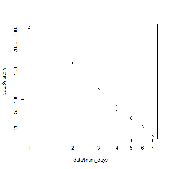
The temporal progress of the numbers strongly reminded me of a power law function, i.e., a function of the form y = a * xb. So I posed myself the following question: How can I determine the parameters a and b from the given empirical data and what will they look like? A quick Google search pointed me to a very helpful StackExchange page. The solution given there was to determine a linear regression model based on a logarithmic scaling of both the x and y axes:
data <- read.csv(file="data.csv")
plot(data$days, data$visitors, log="xy", cex=0.8)
model <- lm(log(data$visitors) ~ log(data$days))
points(data$days,
  round(exp(coef(model)[1] + coef(model)[2] * log(data$days))),
  col="red")

Actual number of visitors (black) vs. fitted model (red), on a double logarithmic scale.
Transforming the Regression Function
The determined model yields two parameters coef(model)[1] =: c and coef(model)[2] =: d. Yet, since the model is a linear regression model, these parameters correspond to the function y = ec + d * ln(x). To obtain the desired form y = a * xb, we can transform the given function as follows:

Results
This means that the parameter a is given by ec while the parameter b is given by d. Thus, they can be obtained using the following assignments in R:

a <- exp(coef(model)[1])
b <- coef(model)[2]

For my data, this gave me the following parameters:
data
c
a
b
regression function
visitors
8.729153
6180.491018
-3.220374
y = 6180.491018 * x-3.220374
views
8.948748
7698.247619
-3.203968
y = 7698.247619 * x-3.203968
To conclude, simple power law regression is not as difficult as it might seem at first. However, in scientific work, it is necessary to also investigate uncertainty in the regression parameters and test the significance of the fitted model. More information on this topic can be found in this paper and on the accompanying website.
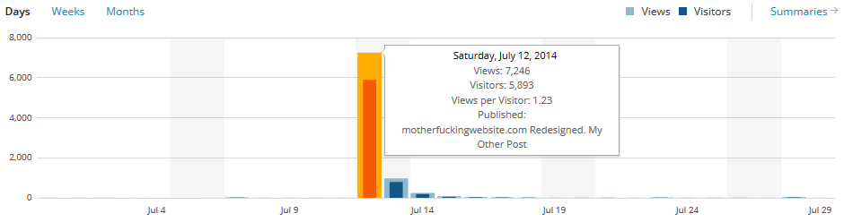 Recently, my post about motherfuckingwebsite.com was featured on the front page of Y Combinator’s Hacker News. I was watching football with some friends when my WordPress app told me twice that my blog’s stats “are exploding”. Back at home, I checked my stats and noticed that I had almost 6,000 unique visitors and over 7,000 views that day (i.e., “day 1”), instead of the normal 4–10 visitors. The effect of the publication on Hacker News was noticeable until day 7, with 13 visitors and 16 views, which was still above average. The number of visitors was back to normal (4 visitors/views) only on day 8.